Yashas's Blog

Optimizing Fibonacci Computation

I posted about this on Twitter yesterday.

I've been attempting to study the topic of algorithms this break because one of my classes next semester will cover exactly that. I came upon an MIT series of lectures for a class named "Introduction to Algorithms", and I reached this video yesterday on dynamic programming.

The professor says that there is a O(log n) algorithm for computing fibonacci numbers, and I'm instantly intrigued. I assumed that O(n) was the best that could be accomplished because all of the fibonacci functions we used in our classes were written that way.

I went to this Wikipedia article and started reading. In particular, they list this formula:

$$ ** \begin{pmatrix} 1 & 1 \\ 1 & 0 \\ \end{pmatrix}**^{n} = \begin{pmatrix} F_{n+1} & F_{n} \\ F_{n} & F_{n-1} \\ \end{pmatrix} $$

I realized that I could use numpy to represent the first matrix, and I could use a loop up to a number n, continuously multiplying a resultant matrix with the first matrix above. This is one way to get a O(n) algorithm.

Here's the code for a linear fibonacci function. I know numpy has a matrix_power() method, but that method is optimized for calculation and doesn't help to demonstrate the linear runtime of the code below.

	import numpy as np

	MATRIX = np.array([[1, 1],
	[1, 0]])

	def linear_fibonacci(num):
	# The matrix above to the nth power will have the nth fibonacci
	# number in its second and third entries.
	result = np.copy(MATRIX)

	for _ in range(num - 1):
	result = np.matmul(result, MATRIX)

	# Could've used: 'return result[1][0]'
	return result[0][1]

view raw linear_fibonacci.py hosted with ❤ by GitHub

Now to make the O(log n) algorithm. These types of algorithms are usually created by splitting the input in half many times. I chose an arbitrary n=10. The exponent rule of

$$ a^n * a^m = a^{n + m} (1) $$

still applies for matrices. Along this line of logic, if we want to compute the fibonacci matrix for n=10, we can multiply two fibonacci matrices of power n=5. That is,

$$ A^5 * A^5 = A^{10} $$

and the second and third entries of the resultant matrix will be our desired fibonacci numbers for n=10. Now we have to figure out a way to find the fibonacci matrix for n=5. Five isn't divisible by two, so we'll have to use a slightly different method. We know

$$ A^2 * A^2 = A^{4} $$

If we multiply the resultant matrix by our base matrix, then

$$ A^4 * A^1 = A^5 $$

We get the desired matrix! So we now have another rule: if the desired matrix has an odd power, we have to multiply two matrices with floor(n / 2) and then multiply once more by the base matrix.

Now we have to figure out a way to start from the base matrix and go up to our desired matrix. Recursion seemed like the best way forward, but I think writing functions iteratively is easier to read, so I'll do it iteratively.

	# We create a stack, floor dividing by 2 each time.
	# The length of the stack determines how many matrix multiplications to do
	stack = [num]
	while stack[len(stack) - 1] != 1:
	last_ele = stack[len(stack) - 1]
	stack.append(last_ele // 2 )

view raw log_fibonacci_stack.py hosted with ❤ by GitHub

In this script, we put 10 into a list. The base case will be where n=1, so we loop and add floor(n / 2) to the list as long as we haven't added one to the end of the list. Here are some examples of what the stack would look like when we finish:

	[10, 5, 2, 1] # n = 10
	[11, 5, 2, 1] # n = 11
	[53, 26, 13, 6, 3, 1] # n = 53

view raw log_fibonacci_stack_examples.py hosted with ❤ by GitHub

Now we create a matrix result. We know all the possible stacks will have a 1 in its last element, so we can just remove it from the stack without losing any information. Now we can process the numbers in the stack. While the stack is not empty, we multiply result by itself. If the number we popped from the stack is odd, then we multiply result by the base matrix.

Here's the code for this part:

	def log_fibonacci(num):
	result = np.copy(MATRIX)

	# We create a stack, floor dividing by 2 each time.
	# The length of the stack determines how many matrix multiplications to do
	stack = [num]
	while stack[len(stack) - 1] != 1:
	last_ele = stack[len(stack) - 1]
	stack.append(last_ele // 2 )

	# The last element, which will be one, does not provide any useful info.
	stack.pop()

	while len(stack) != 0:
	result = np.matmul(result, result)

	# If smallest integer is odd, then we multiply by MATRIX once more
	# to match the necessary power on result
	if stack.pop() % 2 == 1:
	# Do one final multiplication in this cycle if we have an odd number
	result = np.matmul(result, MATRIX)

	return result[0][1]

view raw log_fibonacci.py hosted with ❤ by GitHub

I wanted to test to see if I implemented these algorithms correctly, so I created another module to time these functions. We can use the timeit module to time small code snippets. By default, timeit will run the code snippet one million times.

Here's the code for the timing part:

	import timeit

	def make_setup_string(num):
	string = "import efficient_fibonacci as fib\n"
	string += f"num = {num}"

	return string

	def main():
	print("\nLinear testing started")

	for num in range(15, 91, 15): # We test 15, 30, 45, 60, 75, 90 as inputs
	comp_time = timeit.timeit('fib.linear_fibonacci(num)', setup=make_setup_string(num))
	print(f'\nLinear fibonacci calculation for n={num} took {comp_time} seconds')

	print("\nLogarithmic testing started")

	for num in range(15, 91, 15): # Again, test 15, 30 ... 90 as inputs
	comp_time = timeit.timeit('fib.log_fibonacci(num)', setup=make_setup_string(num))
	print(f'\nLogarithmic fibonacci calculation for n={num} took {comp_time} seconds')

	print()

	if __name__ == '__main__':
	main()

view raw timing_fibonacci.py hosted with ❤ by GitHub

The code snippet inside timeit.timeit() has to be self-contained. It cannot use any external variables. We can, however, pass in a string containing commands that will setup the environment for the code snippet to work. We can use the make_setup_string() function for this purpose.

My final results, as I also posted on Twitter, are shown here:

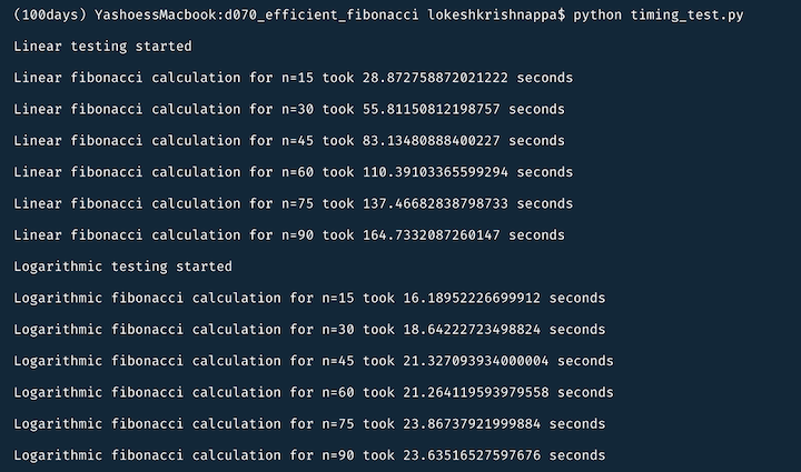
Image of the timing results, you can look on Twitter if you can't view it here using the link above.

The timing for the linear_fibonacci() function increases by about 28 seconds every increase of 15 to the input, so we accomplished a linear, or O(n) algorithm.

The timing for the log_fibonacci() function does not follow this same trend. For n=60 and n=90, the timings are lower than the next lower value of n. Even with the input size increasing linearly, there is not a large change in the timing, so we implemented a correct O(log n) algorithm for finding fibonacci numbers.

Thanks for reading! Follow me on Twitter or look at some of my other work on GitHub by clicking on the social links below.